After a bunch of heavy projects like Tron Cycle, Intelligence Question, TSP, Electronic Life, I wanted to do a few quick and easy pages. Holi Special, Mandelbrot Set, were the results. Next I found a video by Daniel on Lorenz Attractor. Just what I was looking for, another quick, easy code and awesome to look at animation.
Then I came across a page by Juan Carlos Ponce Campuzano which had additional interesting attractors. Suddenly the easy page became a small project of its own. No regrets though. From Juan's page it was evident that a lot of research has been put in to showcase so many attractors. I was lucky to have that as a reference, because the systems are very sensitive to the constants and the initial starting point. Small differences here and there and it would result in a very different curve with little to no resemblance to any attractors here.
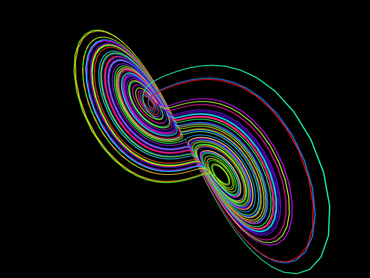
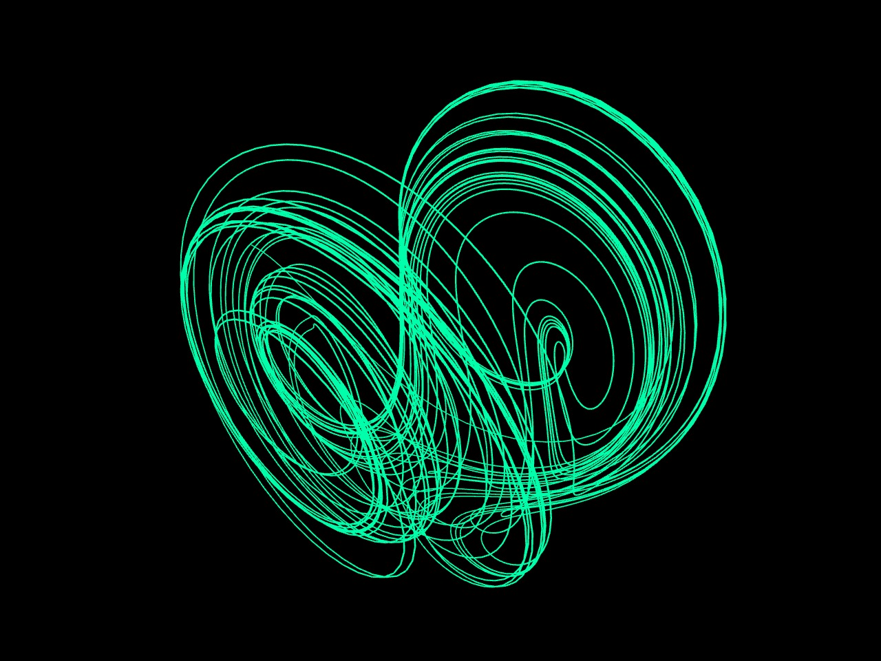
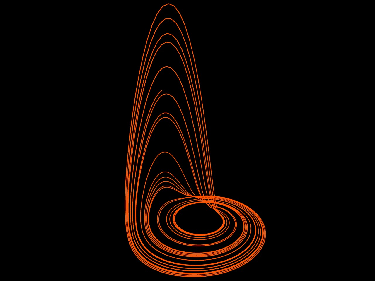
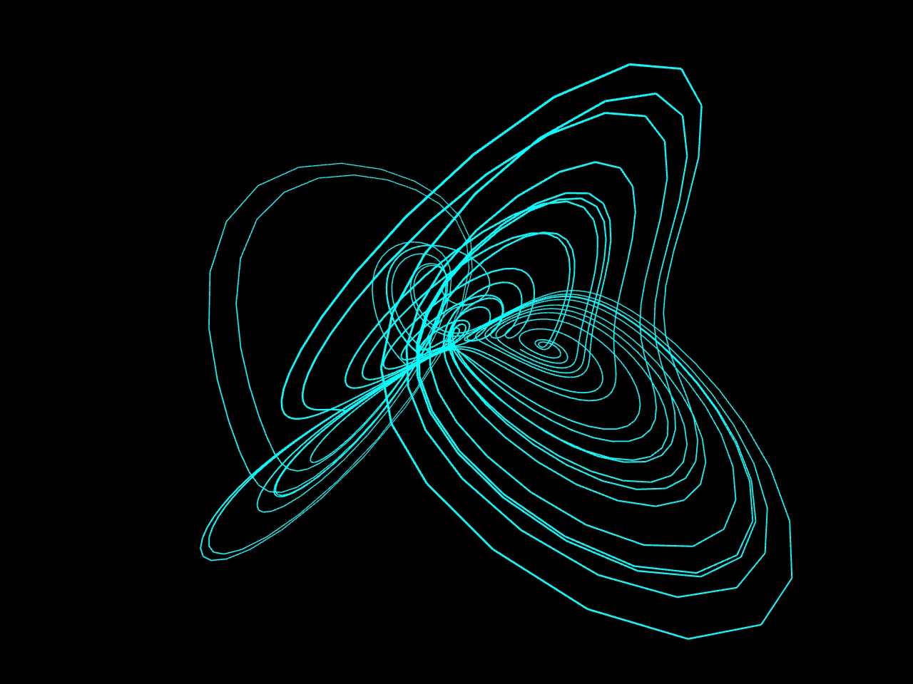
The Attractors
- dx⁄dt = σ(−x + y)
- dy⁄dt = −xz + ρx − y
- dz⁄dt = xy − βz
where σ = 10, ρ = 28, β = 8⁄3
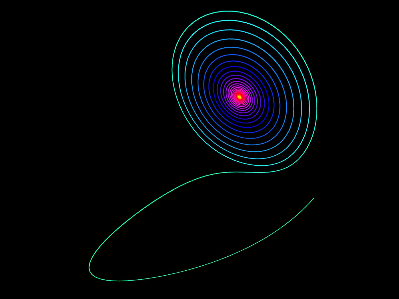
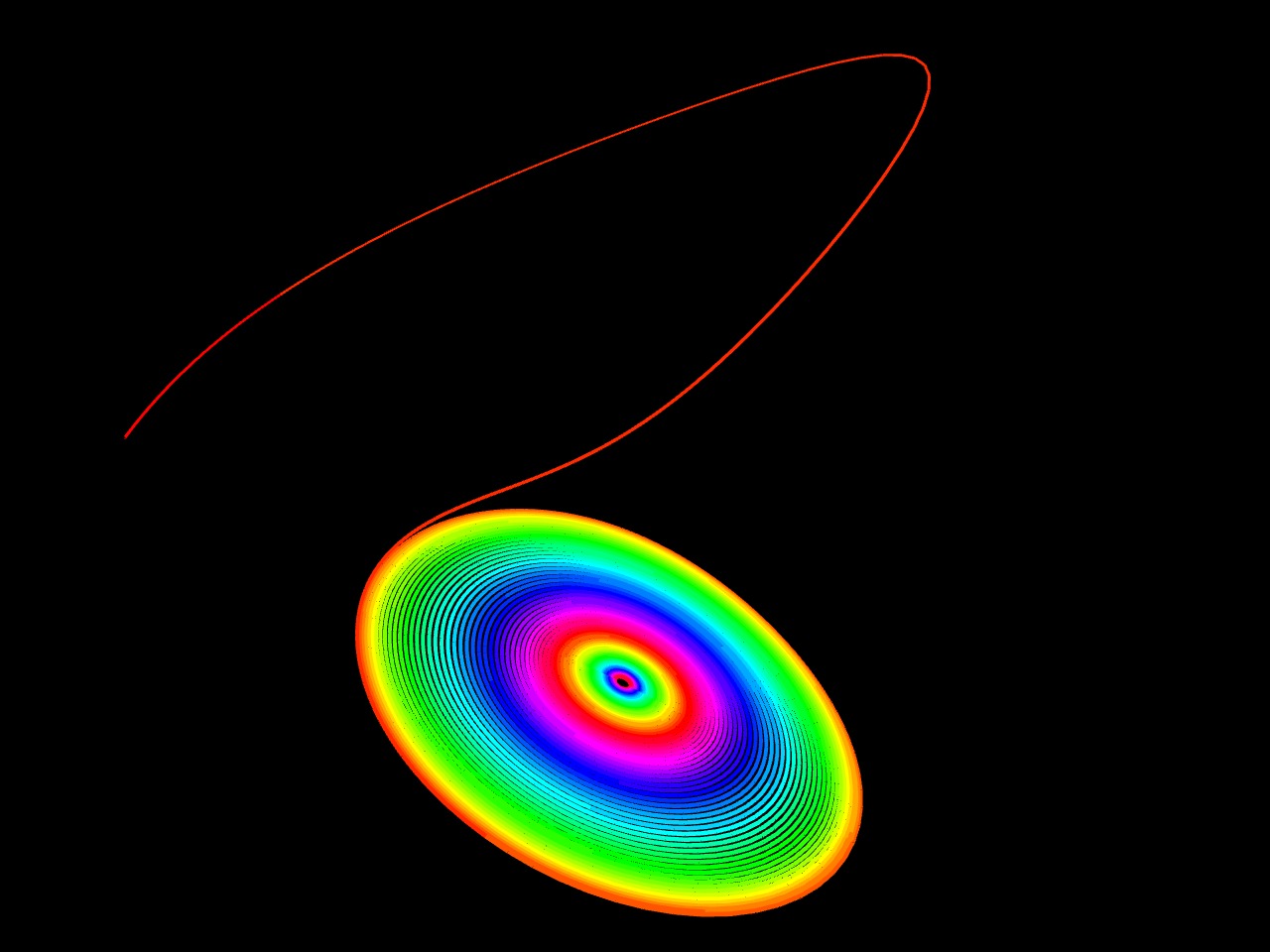
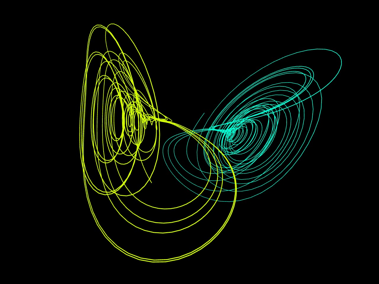
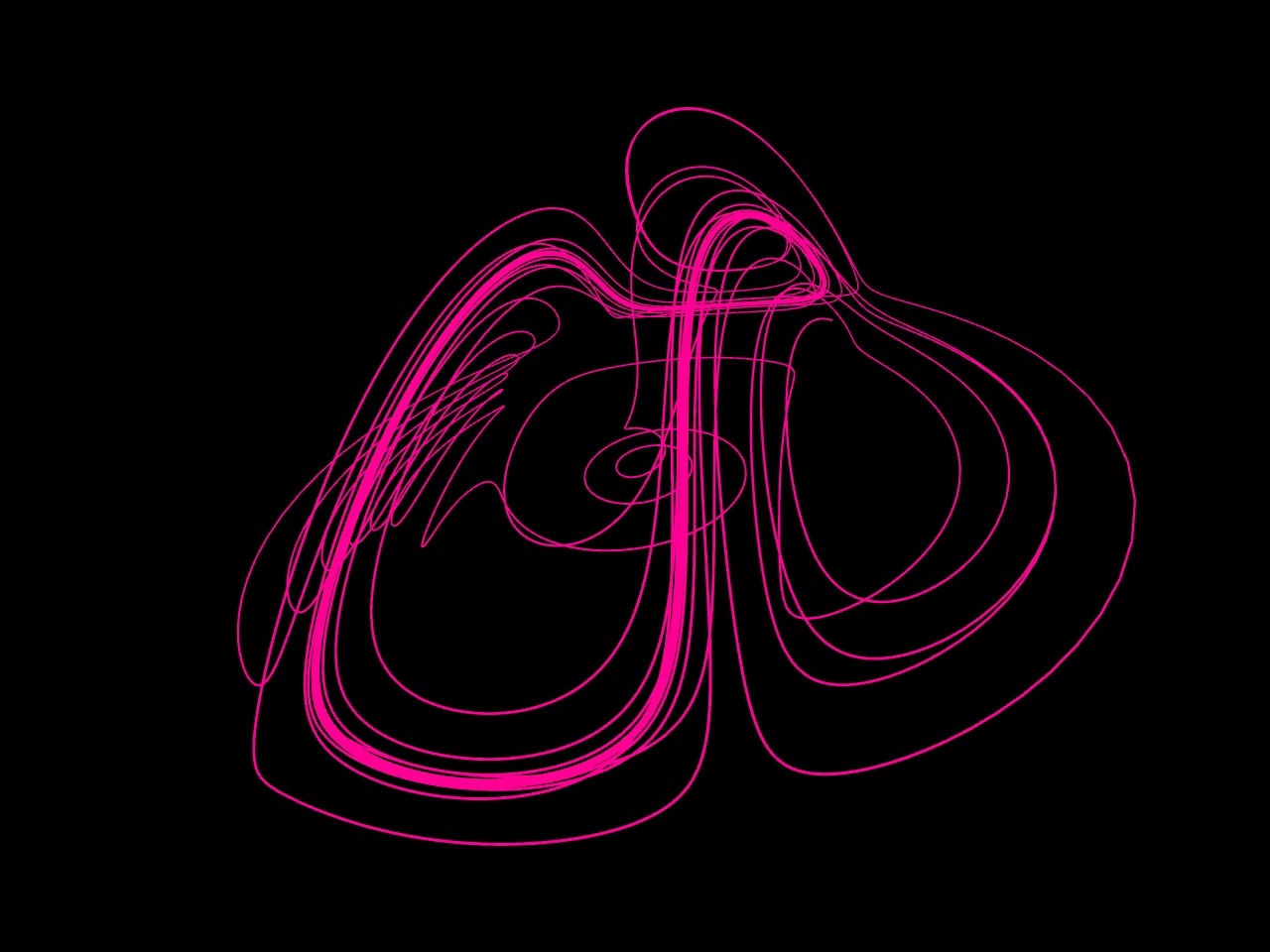
In the same equations, change in constants results in very different curves.
σ = 10, ρ = 14, β = 8⁄3
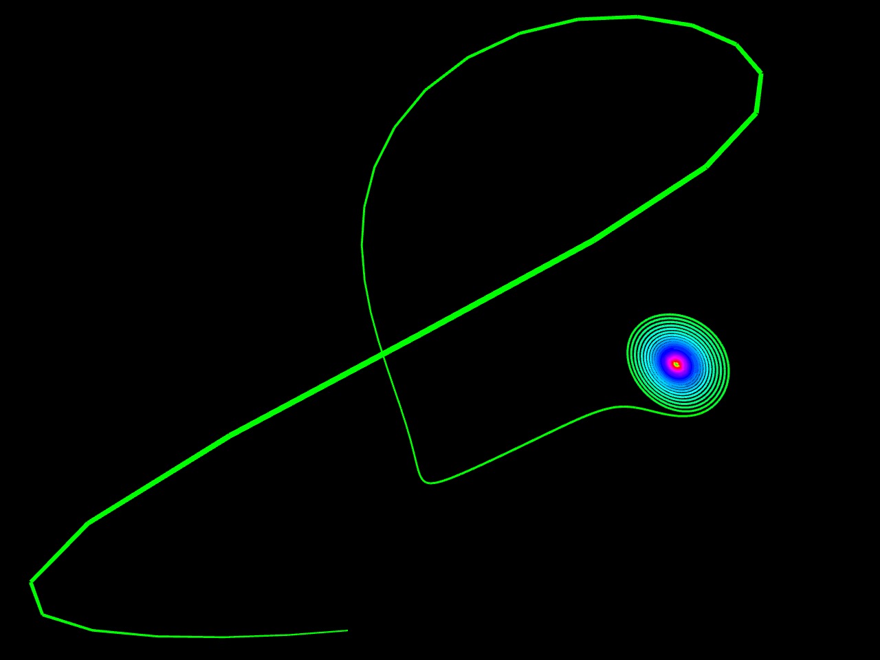
σ = 10, ρ = 13, β = 8⁄3
σ = 10, ρ = 15, β = 8⁄3
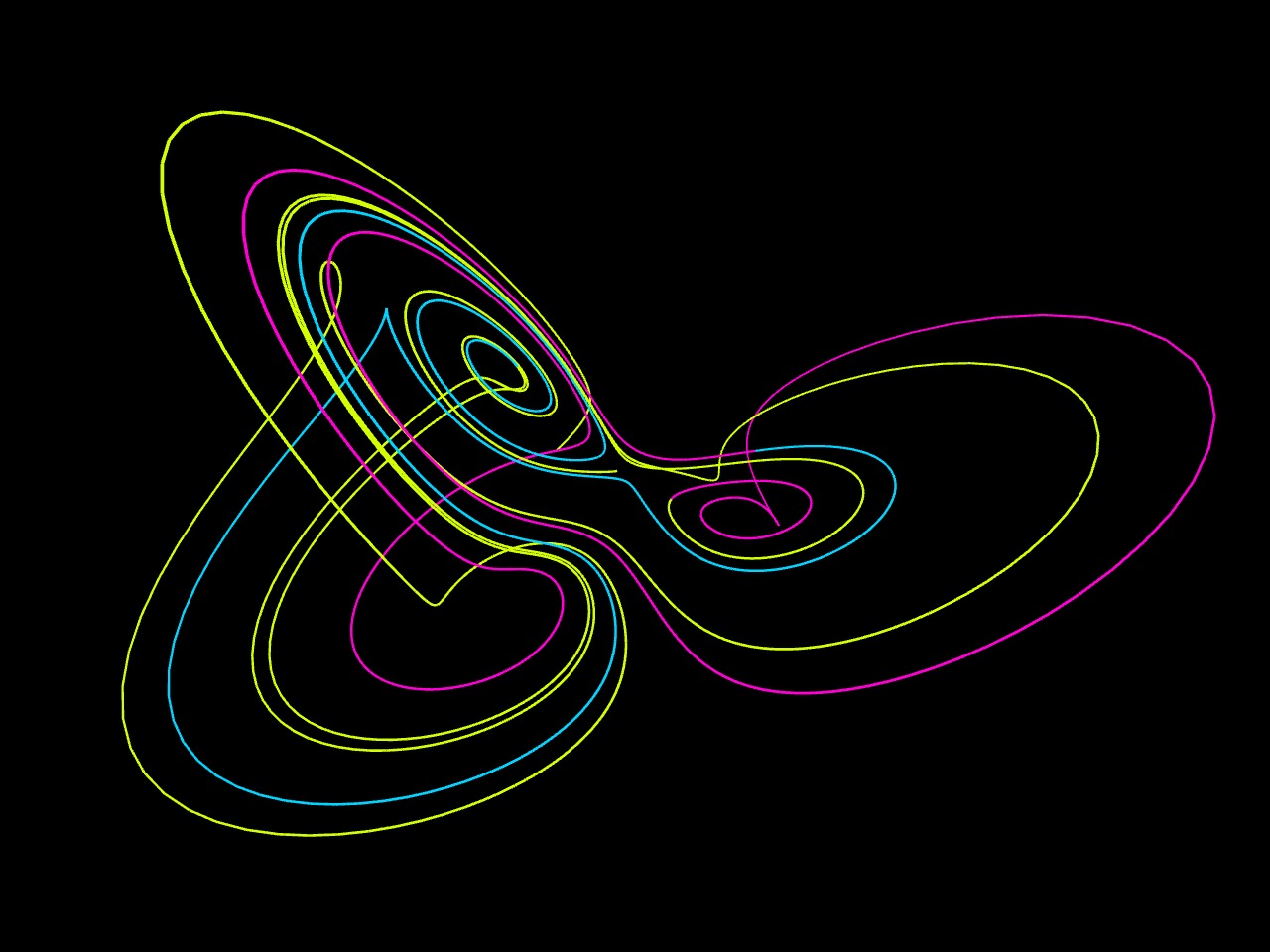
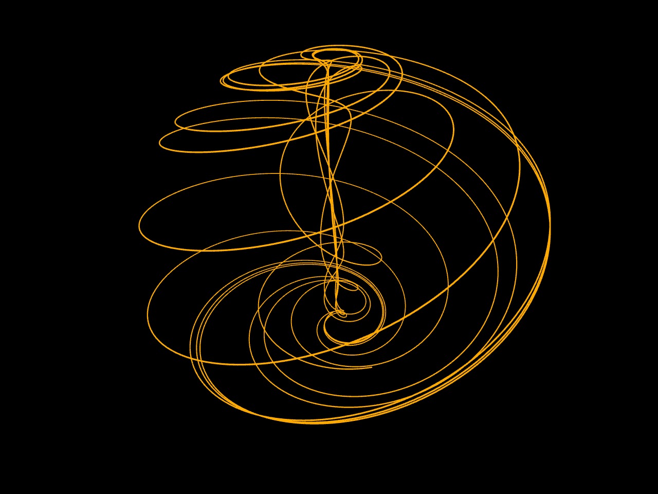
- dx⁄dt = −ax − y2 − z2 + af
- dy⁄dt = −y + xy − bxz + g
- dz⁄dt = −z + bxy + xz
where a = 0.95, b = 7.91, f = 4.83, g = 4.66
Note that two curves are drawn here with different initial points.
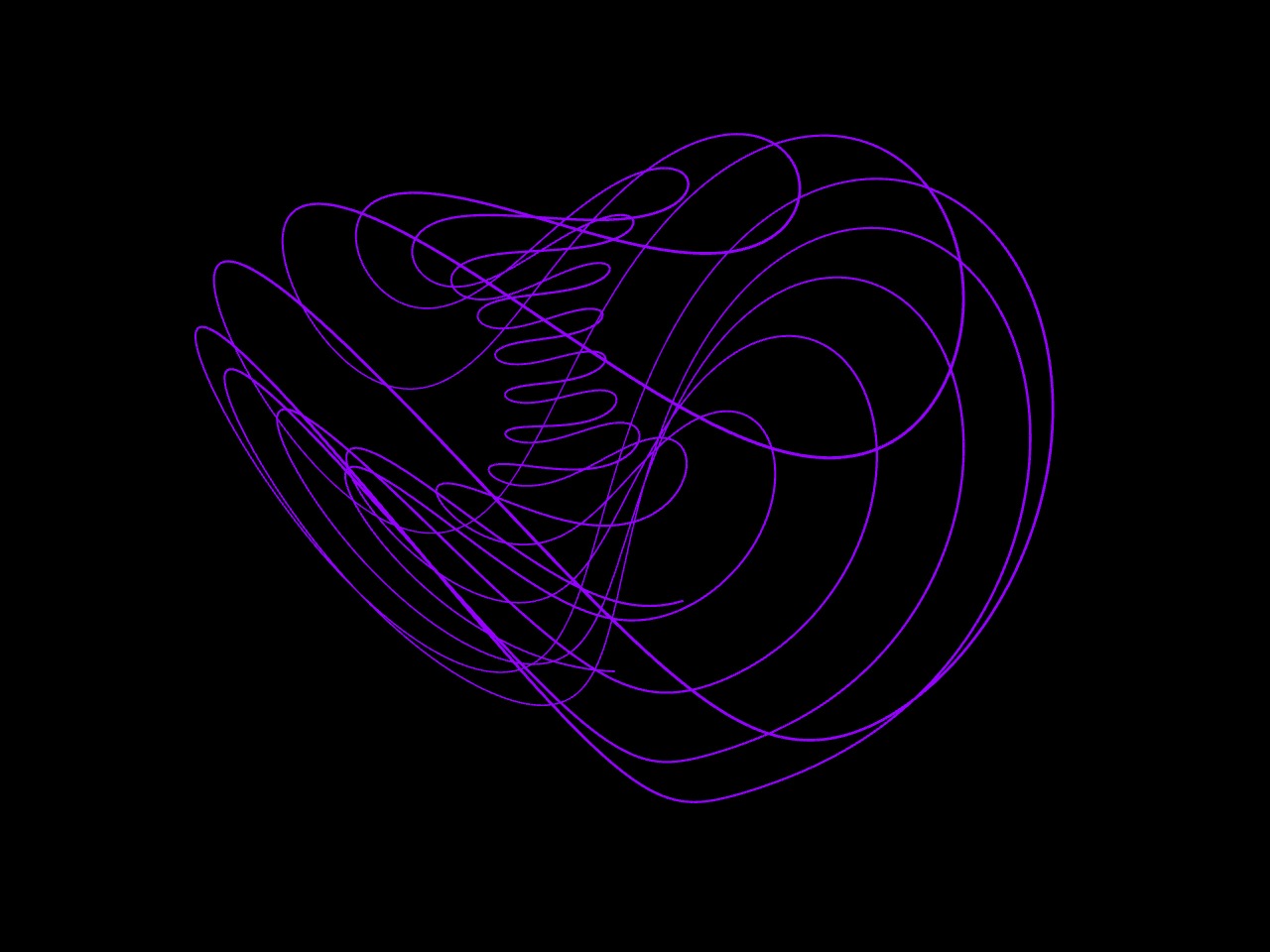
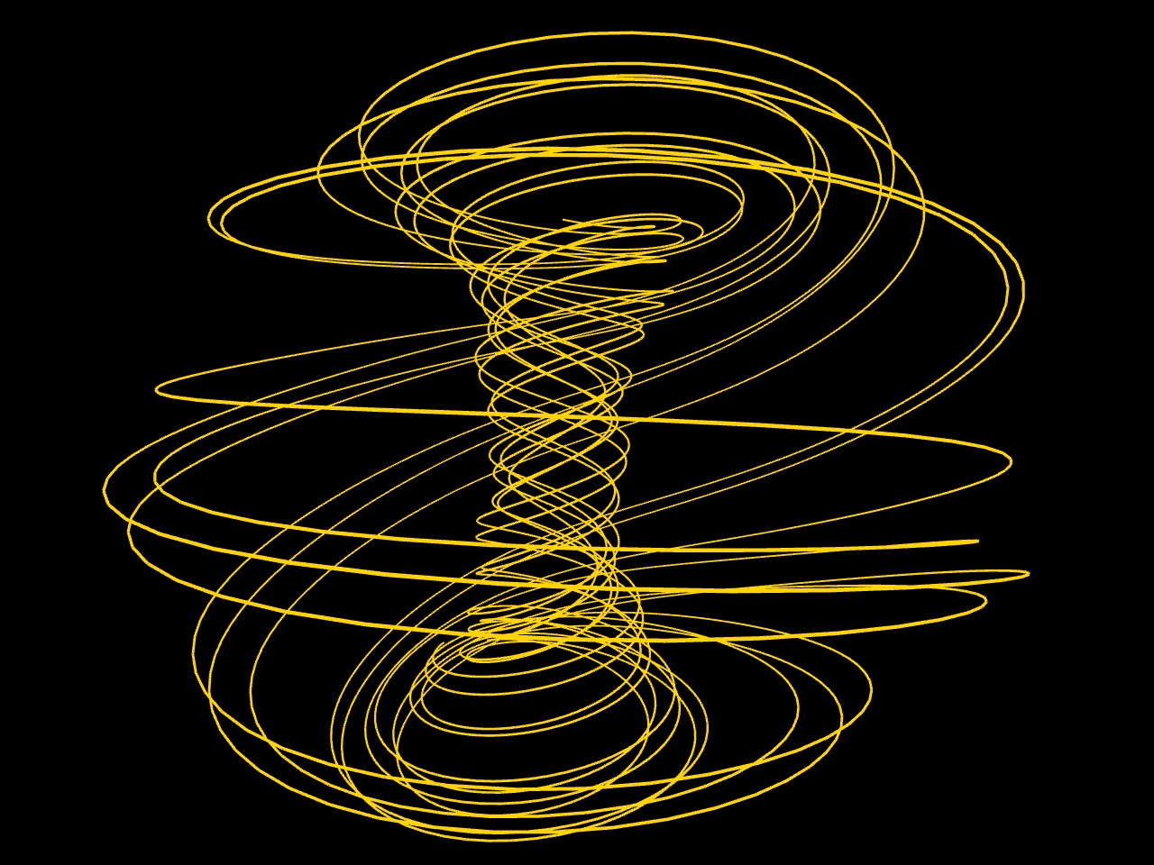
- dx⁄dt = αx − yz
- dy⁄dt = βy + xz
- dz⁄dt = δz + xy⁄3
where α = 5, β = −10, δ = −0.38
- dx⁄dt = y − ax + byz
- dy⁄dt = cy − xz + z
- dz⁄dt = dxy − ez
where a = 3, b = 2.7, c = 1.7, d = 2, e = 9
- dx⁄dt = sin y − bx
- dy⁄dt = sin z − by
- dz⁄dt = sin x − bz
where b = 0.208186
- dx⁄dt = (z − b)x − Dy
- dy⁄dt = Dx + (z − b)y
- dz⁄dt = c + az − z3⁄3 − (x2 + y2)(1 + ez) + fzx3
where a = 0.95, b = 0.7, c = 0.6, D = 3.5, e = 0.25, f = 0.1
- dx⁄dt = −(y + z)
- dy⁄dt = x + ay
- dz⁄dt = b + z(x − c)
where a = 0.2, b = 0.2, c = 5.7
- dx⁄dt = −ax − 4y − 4z − y2
- dy⁄dt = −ay − 4z − 4x − z2
- dz⁄dt = −az − 4x − 4y − x2
where a = 1.89

- dx⁄dt = y(z − 1 + x2) + γx
- dy⁄dt = x(3z + 1 − x2) + γy
- dz⁄dt = −2z(α + xy)
where α = 0.14, γ = 0.1
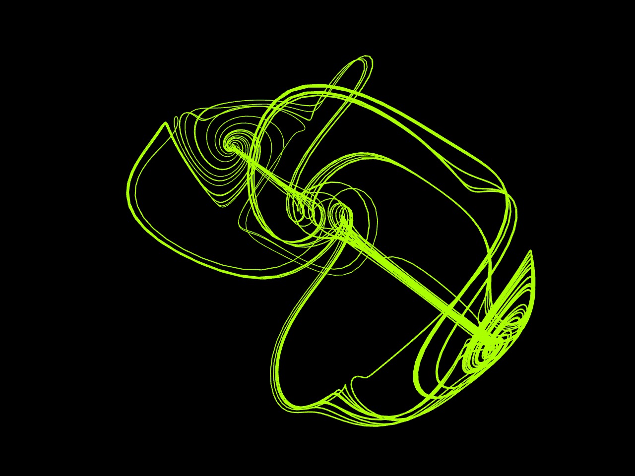
Three-Scroll Unified Chaotic System
- dx⁄dt = a(y − x) + dxz
- dy⁄dt = bx − xz + fy
- dz⁄dt = cz + xy − ex2
where a = 32.48, b = 45.84, c = 1.18, d = 0.13, e = 0.57, f = 14.7
- dx⁄dt = y + axy + xz
- dy⁄dt = 1 − bx2 + yz
- dz⁄dt = x − x2 − y2
where a = 2.07, b = 1.79
- dx⁄dt = ax + yz
- dy⁄dt = bx + cy − xz
- dz⁄dt = −z − xy
where a = 0.2, b = 0.01, c = −0.4
Controls
Select a system.
Animation speed controls how fast (or slow) the Sysytem will get generated.
Using mouse on the Viewport allows to control the camera. I have used p5.EasyCam for the 3D camera here.
Camera controls - straight from EasyCam site
- To rotate around the look-at point, left-click and drag.
- To pan the scene, middle-click and drag
- To zoom out/in, right-click drag
- To reset to the starting state, double-click